Summary of our pilot Soil Vegetation Map digitization project in Sonoma County

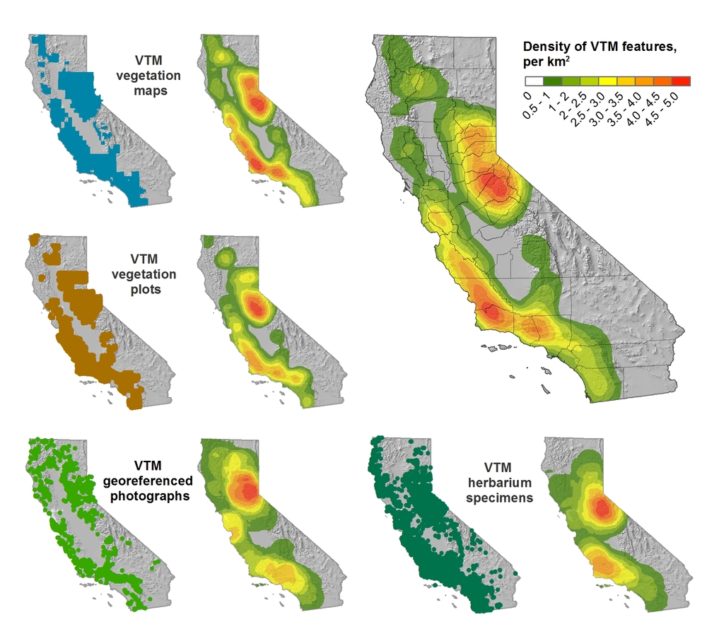
Between the years 1949-1979 the Pacific Southwest research station branch of the U.S. Forest service published two series of maps: 1) The Soil-Vegetation Maps, and 2) Timber Stand Vegetation Maps. These maps to our knowledge have not been digitized, and exist in paper form in university library collections, including the UC Berkeley BioScience and Natural Resources Library.

Collection Description

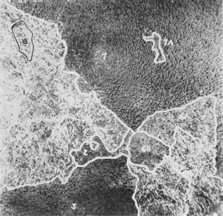
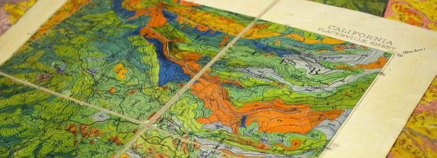
The Soil-Vegetation Maps use blue or black symbols to show the species composition of woody vegetation, series and phases of soil types, and the site-quality class of timber. A separate legend entitled “Legends and Supplemental Information to Accompany Soil-Vegetation Maps of California” allow for the interpretation of these symbols in maps published 1963 or earlier. Maps released following 1963 are usually accompanied by a report including legends, or a set of “Tables”. These maps are published on USGS quadrangles at two scales 1:31,680 and 1:24,000. Each 1:24,000 sheet represents about 36,000 acres. See Figure 1 for the original index key.

The Timber Stand Vegetation Maps use blue or black symbols to show broad vegetation types and the density of woody vegetation, age-size, structure, and density of conifer timber stands and other information about the land and vegetation resources is captured. The accompanying “Legends and Supplemental Information to Accompany Timber Stand-Vegetation Cover Maps of California” allows for interpretation of those symbols. Unlike the Soil-Vegetation Maps a single issue of the legend is sufficient for interpretation. See Figure 2 for the original index key.

Methods

We found 22 quad sheets for Sonoma County in the Koshland BioScience Library at UC Berkeley.

Scanning

Using a large format scanner at UC Berkeley’s Earth Science and Map library we scanned each original quad at a standard 300dpi resolution. The staff at the Earth Science Library completes the scans and provides an online portal with which to download. Current library recharge is at $10 per quad sheet. Coordinating the release of the maps from the UC Berkeley BioScience library and subsequent transfer to the UC Berkeley Earth Science and Map library currently requires a UC member with valid library privileges to check out the maps. 

Georeferencing

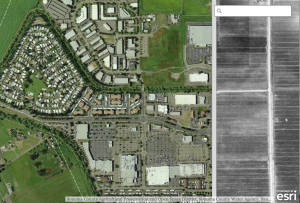
Georeferencing of the maps was done in ArcGIS Desktop using the georeferencing toolbar. For the Sonoma county quads which are at a standard 1:24,000 scale we were able to employ the use of the USGS 24k quad index file for corner reference points to manually georeference each quad. We used Upper Right, Upper Left, Lower Right, Lower Left as our tie points. The USGS quads are projected in polyconic NAD 1927 UTM Zone 10 projection so we adjusted our data frame to match this original projection and register the image. For a step by step description of this process see “Georeferencing Steps in ArcMap”.

Error estimation

The georeferencing process of historical datasets often produces error. We capture the error created through this process through the root mean squared error (RMSE). The min value from these 22 quads is 4.9, the max value is 15.6 and the mean is 9.9. This information must be captured before the image is registered. See Table 1 below for individual RMSE scores for all 22 quads. 

Table 1: Quad original name, quad name from the downloaded USGS 24k file, and the RMSE of the georeferencing process. 

Quad Name                      Quad Name                    RMSE (m)

60A-3                                Whispering Pines            7.48705

60B-3                                Asti                                 12.7461

60B-4                                The Geysers                    6.84357

60C-1                                Jimtown                          7.66811

60C-2                                Geyserville                      6.60752

60C-3                                Guerneville                     14.8663

60D-12                              Mount Saint Helena       10.7671

61A-3                                Big Foot Mountain          9.77075

61A-4                                Cloverdale                      9.37442

61B-3                                McGuire Ridge               7.90499

61B-4                                Gube Mountain              15.3223

61C-1                                Annapolis                       5.66674

61C-2                                Stewarts Point                 14.8612

61C-4                                Plantation                       4.91229

61D-1                                Warm Springs Dam         15.562

61D-2                                Tombs Creek                   12.995

61D-3                                Fort Ross                         9.06434

61D-4                                Cazadero                        13.0045

62A-4                                Gualala                          11.1405

63A-1                                Duncans Mills                 7.44373

63A-2                                Arched Rock                   5.55524

64B-2                                Camp Meeker                 8.91102

Aerial photography archives

Notes on where to find historical aerial imagery (thanks to Kass Green): The USDA has an archive of aerial imagery in Salt Lake City at APFOhttp://www.fsa.usda.gov/programs-and-services/aerial-photography/index.  There is a ArcGIS online map of the  tiles and dates of this photos. Search in ArcGIS online for the AFPO Historical Availability Tile Layer. USDA is in the process of scanning these photos, but you can order them through a manual process now (which can take a long time). 

The EROS data center in Sioux Falls also has an archive of high altitude photos for the US from the 1980s.  Also check out https://lta.cr.usgs.gov/NHAP  and https://lta.cr.usgs.gov/NAPP .  These photos are available digitally, but are not terrain corrected or georeferenced.

ISECCI historical ecology working group wrap-up

Last week Kelly and I with others travelled to the Sierra Nevada Aquatic Research Lab (SNARL) in the eastern Sierra Nevada, just south of Mono Lake for a research retreat. SNARL is part of the UC's Natural Reserve System, which is comprised of nearly 40 properties across the state. These are preserves that foster research, education and collaboration. They have much in common with ANR's REC system. I've been to a few of them now, and am very pleased to make more visits. I love the east side of the Sierra, and that iconic Highway 395. 

This trip was a retreat for the ISECCI historical ecology working group, led by the inspirational Peter Alagona from UCSB. We discussed our existing projects, including the VTM work (see figure below), and talked about potentials for more collaborative research and further integration between NRS and ANR. We have a list of wishes for digitization, and if anyone out there has ideas about pitching these to donors, please let me know. For example: 

  • Kelly and I want to digitize the Leiburg maps from the northern Sierra to add to the VTM stack;
  • We want to find a better way to index and view historical aerial photography state-wide. Something like this for historical maps: http://ngmdb.usgs.gov/maps/TopoView/help/

And we had a field trip looking at Mono Lake water issues. Great time spent!

Density of VTM features across the collections

Robert Colwell Musings Part 2

I started this last year when I was working on a retrospective of remote sensing of forests in California for the centennial of Berkeley Forestry. In the article I tried to highlight some of the pioneering work done by remote sensors that focused on Californian forests from the 1960s through the use of lidar today. As is often the case, the paper changed into something a bit more focused on lidar technology, and I had to cut most of the Colwell stuff. So, I reprise some information about him here, add my perspective on his work as antecedants to modern OBIA approaches, and include his rad interior design ideas. 

Early musings on forest objects by Colwell in 1964.

Dr. Colwell was an internationally renowned remote sensing scientist; he was former associate director of the Space Sciences Laboratory at the UC Berkeley, and he was the instructor of remote sensing in our own Mulford Hall from 1947 until his retirement in 1983. He was NASA co-investigator for Apollo IX, and his research in the 1960s on reflectance and multispectral reconnaissance were the primary basis for selecting the type of sensors and the spectral bands implemented in Landsat. Neat guy, and we all benefit from his intellectual legacy.

Finding meaningful blobs - a geographer’s quest

In our new Taylor and Francis book chapter, Thomas Blaschke, Helena Merschdorf, and I discuss Object-Based Image Analysis: Evolution, History, State of the Art, and Future Vision (Book website).  I did some work looking into Colwell's work, and found lots of discussion of nascent work describing object based approaches to image analysis. He struggled with the inability of algorithms to pull from digital imagery meaningful "blobs". See the examples here. 

One of Colwell's early attempts at object based work from 1973. Printout on a dot matrix printer?

His assessment of the potential for automation of an object recognition process depended on the capacities of a digital scanner and the ability of an algorithm to assess the differences, in photographic tone, between a "blob" and its surroundings (Colwell 1964, 1965). Colwell was an important advisor on the Landsat 1 mission, and his ideas on extraction of meaningful features transferred to his ambitions for the satellite missions (Colwell 1973). 

Maps as hipster decorations

I read some of his work as he transitioned from aerial photography to digital imaging, and I came across this picture. Mulford is just off the scene in the upper left corner, and Hearst Gym pool is visible in lower part. 

Oblique aerial view of Berkeley Campus of University of California taken with Camouflage Detection film. Robert N. Colwell

In his caption he says:

"Oblique aerial view of Berkeley Campus of University of California taken with Camouflage Detection film."(That is what they used to call color infrared.) "Such photography is superior to any other for certain photo interpretation purposes as indicated by some of the preceding examples. Note in this photo how color values for each species of tree tend to remain uniform from foreground to background because of the superior haze penetration offered by this film. The relatively long wavelengths to which this infrared-sensitive film reacts are scattered but very little by atmospheric haze particles, thus accounting for the uniform color values and for excellent image sharpness." I dig this part: "The original color transparencies have the same color values as seen here and consequently make very attractive panels for lamp shades, although certain of their colors fade upon prolonged exposure to light."

The trend for using map products as kitchy home decorations PRE-DATES 1970! Take that hipsters!

Articles mentioned:

Colwell, R.N. 1964. Aerial photography - A valuable sensor for the scientist. American Scientist, Vol. 52, No. 1 (MARCH 1964), pp. 16-49

Colwell, R.N., 1973. Remote Sensing as an Aid to the Management of Earth Resources. American Scientist. 61(2): 175-183.

Some more about him here: http://senate.universityofcalifornia.edu/inmemoriam/robertcolwell.htm

Historical data and the NRS

Just got off a call with a group of people focusing on historical data discovery at the Natural Reserve System (NRS). This process is part of the recently funded Institute for the Study of Ecological Effects of Climate Impacts (ISEECI). People in the group include:  

Of particular note was the introduction of the Online Archive of California, which is a collection of metadata about historical archives. Peter is adding all his data to the OAC. His work was funded through a Research Opportunity Fund grant through UCOP, and a NSF grant.  The process the NRS has used is different than what we have done with the REC data. They have assembled metadata from the research reports from the stations, and full digitization can be opportunisic and focused on particular questions. There is a Zotero database of publications that have resulted from the reserves. 

Other important links:

The metadata data from research applications submitted through RAMS - tends to be incomplete as we rely on PI's to proof the entry and then submit it. 

http://nrs.ucop.edu/MetaData.htm

The reference database, this has had extensive work done on it, and should be fairly complete. Lynn's working on a complementary database for Santa Cruz Island historic data, which will be made available. 

http://nrs.ucop.edu/bibliography.htm

Climate data - currently hosted on DRI's website, and data should be available for download.

http://www.wrcc.dri.edu/ucnrs/index.html

10-year anniversary for the GIF

I'm musing, contemplating and writing on the decade 2005-2015, as this is the GIF's 10-year anniversary. What a decade it was. Here I'll post and add to some of the key events that helped transform mapping (and the GIF) in the last 10 years.

Key background events

  • 1996. Mapquest launched.
  • 1997. Skynet becomes self-aware.
  • May 2000. Selective Availabilility on GPS turned off, leading the way for GPS in smartphones.
  • The Scan Line Corrector (SLC) on the Landsat 7 ETM+ instrument failed May 31, 2003.
  • 2004. Open Street Map founded.
  • March 2004. Yahoo! maps launched, first slippy maps (click and drag to pan and zoom the map).
  • 2004. NASA releases WorldWind.
  • October 2004. Google acquires Where 2 allowing AJAX map tiling to a desktop client.
  • October 2004. Google acquires Keyhole.

What made 2005 such a crazy year

  • Google Maps launches in February, and goes mobile in April.
  • The first mashup: Paul Rademacher's Housingmaps.org. His original post on Craigslist asking for feedback: https://forums.craigslist.org/?ID=26638141
  • Google Maps API launches in June.
  • NASA's Blue Marble Next Generation released.
  • Google Earth launches in June.
  • Hurricane Katrina hits in August. Simple webmaps for the disaster proliferate, and ESRI and GE get on the scene.
  • Kellylab's first blog post in September.
  • GIF launches and hosts our first GIS Day in November with Michael Jones, formerly of Keyhole.
  • The back-up solar array drive on Landsat 5 began failing and was not able to provide the power needed to charge the batteries. November 26.

Where we are in 2015

We've gone through a number of transitions in the world of mapping:

  • Data have transitioned from being siloed, and found in clearinghouses to being open and provided through APIs.
  • We’ve moved from desktop computing to cloud computing.
  • Webmaps have transitioned from using proprietary stacks to networks with multiple open and proprietary options.
  • We’ve moved from imagery gathered monthly or seasonally to daily; footprints are smaller, and our focus has shifted from local focus to global coverage.
  • Our planimetric 2D view is changing with lidar and radar sensors.
  • Visualization has moved from static cartography or simple animations to dynamic interactive visualization.
  • Finally, mapped content is no longer anonymous or regulated, but highly personal and narrative.

Key GIF milestones:

  • 2005 GIIF (Geospatial Imaging and Informatics Facility) launches
  • 2006 OakMapper changes from ArcIMS to Google Earth API
  • 2008 GIIF becomes GIF
  • 2008 OakMapper 2.0 launches
  • 2008 SNAMP website launches
  • 2011 Cal-Adapt goes live
  • 2013 EcoEngine/HOLOS goes live
  • 2014 LandCarbon launches
  • 2014 GIF and Cal-Adapt go to the White House
  • 2014 vtm.berkeley.edu goes live, built from the HOLOS API
  • 2015 Spatial Data Science bootcamp in May

Onwards and upwards!

100 Years of National Geographic Maps: The Art and Science of Where

Great retrospective on 100 years of National Geographic map making. 

100 Years of National Geographic Maps: The Art and Science of Where

Since 1915, National Geographic cartographers have charted earth, seas, and skies in maps capable of evoking dreams.

This beaut on the right is from 1968 of the ocean floor.  The article says: " Based on the work of geophysicists Bruce Heezen and Marie Tharp, this 1968 map of the ocean floor helped bring the concept of plate tectonics to a wide audience. Tharp began plotting the depths in 1950 from soundings taken by ships in the Atlantic, but, as a woman, wasn't allowed on the ships herself. In 1978 she was awarded the Society's Hubbard Medal for her pioneering research." 

Sonoma County's historic aerial photographs

As part of the massive ongoing effort to map Sonoma County with high-res imagery and lidar, historic imagery of the county was collected and georeferenced. The Sonoma County Agricultural Preservation and Open Space District funded SFEI to mosaic 72 historic aerials taken over Sonoma County by the Department of Defense in 1942. Mark Tukman put together this web service with a image swiping tool showing the combination of the 2011 imagery service and the mosaiced historic imagery.
 
Sonomaopenspace.maps.arcgis.com

About the historic imagery: In 1942, the Department of War collected air photos in anticipation of a possible strike.  These photos are the earliest complete image set for Sonoma County and give us an unprecedented look at Sonoma County's agriculture and open space prior to the post World War II baby boom.

These images are snaps from the service, both from an area outside Rohnert Park in Sonoma County: on the left is the image from 1942, on the right is the area in 2011 showing considerable development.

2011 image

1942 aerial

NEW VTM Reshoot!

Take a look at this awesome VTM reshoot from the folks over at Geographic Resource Solutions (GRS), photographed during a recent mapping project of Lassen Volcanic National Park. Yet another great example and an incredible testament to lasting power of the VTM dataset. This particular photo was taken near the Chaos Crags Jumble in Lassen Volcanic National Park. Thanks to Ken Stumpf and GRS for sharing!

Albert Wieslander (October 1, 1925): Looking N 35 degrees W from 1/4 corner 16/17 T 31-4. Foreground dwarf timber on glacial deposit. Slope in background, section 7 and 8 Tyler Brown of GRS (September,2011): At Accuracy Assessment Site 091646 located in the Chaos Crags Jumble in Lassen Volcanic National Park

In a similar vein I recently stumbled upon another meshing of historical and contemporary photographs. The project features reshoots of the Grand Canyon and resulted in a 2012 book titled: Reconstructing the View: The Grand Canyon Photographs of Mark Klett and Byron Wolfe

Published by University of California Press. You can see a few of the photographer’s recent projects on their website. Historical photos are just the best!


Rescuing historic data for modern use: a cautionary tale from the past

An example of a VTM vegetation map, from Shufei LeiWe have been talking recently with the HOLOS project and the IGIS InfoBase project about the need to "rescue" data and to provide frameworks for data synthesis. I present to you a profound example of these needs: the VTM project. We have launched the new VTM website, in which the maps, plots, and photograph portions of the VTM collection are united and powered by HOLOS, open data, and sharing. The journey from paper collection to digital data has been a long one, with several cases of almost accidental and purposeful destruction. As such it is a cautionary tale about the importance of rescued and shared historical data in ecological and geographical analysis. We owe much to all the people who have contributed to the preservation and digitization of this important collection.

I spent this evening reading the oral history conducted in 1985 by Ann Lange of Albert Wieslander. It is called: California Forester: Mapper of Wildland Vegetation and Soils A. E. Wieslander, and it is a fascinating read. In addition to being a real spitfire and having very clear opinions on things (and people), he also tells this tale about the near loss in 1952 of the vegetation maps. Wieslander had made 23 of his vegetation maps available for publication through the University Press, for production and sale at a cost of $1 each. This was meant to supply funds for the rest of the maps to be published. But that didn't work out as planned.

"Not very many of the maps were sold, even though articles were written to give them publicity. I realized fairly soon that we wouldn't be able to publish any more unless we got additional money someplace.” He was "casually told one day that the University Press had written a letter to the station saying that the maps weren't selling very well, and it wanted to return the quadrangles to the station. They didn't want to handle it anymore.” A forest service employee "told the University Press the station didn't want the maps back and authorized it to dump them. I didn't know anything about this until after it was done. There was nothing I could do about it then. Imagine all these beautiful maps. They didn't even take out one as a sample.”

What!! That is so shortsighted… Anyway read on…

Wies (he refers to himself "Wies" in the interviews) then found out that the University Press couldn't understand the dumping of all those maps and alerted Paul Zinke, Forestry Professor here at Berkeley.

"So Zinke went down and got twenty copies of each of the quadrangles.”

But, we still had all the original field maps, kept at the experiment station. Just before I retired, I talked with Herbert Mason about all the printed maps having been destroyed and about how it was important to preserve the originals. Researchers could use them. He suggested that the Botany Department set up in the Life Sciences Building a plant geography room. And the main feature of this plant geography room would be the vegetation mapping project. So I moved all the files of maps and sample plots over to the Life Sciences Building. Mason went through the material and found at least a third, maybe more, of the original maps were gone.” Apparently, different national forests had been writing to the station requesting certain maps. Since they didn't have any of the printed maps, originals were sent out, with no record kept of what was sent, or to whom. 

This explains why the maps have been scattered across the state, and why it has taken so long to pull them (mostly) together again. 

"The maps then made a trip back to the station, where Dr. William Critchfield used them to write a publication called "The Profiles of California Vegetation”. "Anyway, I'm glad that was done. It was a very nice publication, and it gave proper credit to the draftsman who did the beautiful job of drafting, and to the project, and to me. Then Critchfield also worked with James Griffen, of the university, and got out another publication on "The Distribution of Trees in California." It was based on the maps and other data we had." When Wies expressed "concern about these maps and Dr. Critchfield said, "I would like to get them deposited in the Bancroft Library." I don't know whether he did it or not, but that's what he told me.”

Thank goodness that they are back on campus in the Marian Koshland Library (and for this we are forever in debt to the wonderful Norma Kobzina), and the plot data, plot maps, vegetation maps, and photographs will be re-united and available for use.

1966 Lunar Orbiter 1 Images of Earth Recovered

comparison of the original Earthrise image as seen by the public in 1966 and the restored image released in 2008Interesting article from Wired on the recovery of forgotten images from the 1966 Lunar Orbiter 1 mission. The images were taken from a probe orbiting the moon and contain images of the surface of the moon and distant Earth including the first high resolution photographs ever taken from behind the lunar horizon of an Earthrise. The images were recovered from analog data tapes at NASA Ames and have not been seen publicly since the original data from the mission was received in the late 1960s and never at such high resolution. The historical images of Earth are now being used to fill in gaps about Earth's climate in the 1960s. For the full story click here.

Cal Forestry turns 100 this year!

Forestry education at UC Berkeley began in 1914 with the “Division of Forestry” in the Department of Agriculture. The Department of Forestry was established in 1939 and the School of Forestry in 1946. Forest Summer Camp, the hallmark of the undergraduate program, began at Quincy, California, in 1915 and moved to Meadow Valley in 1917.

Today, alumni of Cal’s forestry program hold critical positions for the management of 95% of the industrial forestlands in California. The research of our alumni and faculty has grown knowledge in the areas of fire, remote sensing and GIS, ecology, climate change, forest economics, the social sciences, and numerous others.

Over the past 100 years, the Cal Forestry program has had an impact on every dimension of the field, and has produced the profession’s most influential thinkers and doers.

For more information, please see: http://nature.berkeley.edu/forestry100/about-us

A great week for radio

What a great week for radio and matters geospatial+web. On Wednesday last week we finished out our GIS class with a talk about the geoweb and issues of access, bias, motivation, control, and of course privacy. I used alot of William Gibson's previous writings about Google (posted here earlier) in that lecture. Yesterday TTBOOK re-aired a great interview with Gibson, on the topic of writing, but also about the internet. I recommend it. Additionally, last week Talk of the Nation had a interesting interview with Jerry Brotton about his new book "A History of the World in Twelve Maps"; the interview touched on Google Earth and representation, why north is up, and many other fantastic questions raised through the history of cartography. Check them out!

Pre-development Delta report from SFEI

The San Francisco Estuary Institute-Aquatic Science Center is pleased to announce the publication of its latest report, Sacramento-San Joaquin Delta Historical Ecology Investigation: Exploring Pattern and Process. The report is the culmination of several years of research synthesizing thousands of pieces of historical evidence with contemporary scientific understanding. The report provides new information about how the Delta functioned to provide habitat for native species and includes dozens of rarely seen historical accounts, maps, and photographs. For more information, please see today's press release.

The report and Geographic Information System (GIS) data are available for download here. Printed copies of the report will be available in several weeks, at a cost of $75 each (plus tax/shipping).

Media Contacts:
Robin Grossinger, Senior Scientist, San Francisco Estuary Institute-Aquatic Science Center, (510) 746-7380 (office), 510 326 3732 (cell), or robin@sfei.org

Carl Wilcox, Policy Advisor to the Director for the Bay-Delta, California Department of Fish and Game, (707) 738-4134, or cwilcox@dfg.ca.gov

One Hundred Years of Land Values in Chicago

Gabriel Ahlfeldt, from the London School of Economics, presents in a video in the link below on an interesting project that digitized Olcott's Blue Books, a unique dataset of historical land values, land uses, building heights, and other information in Chicago and its suburbs, published annually between 1900 and 1990. The digitized information from the Blue Books allows for detailed historical statistical and geospatial analyses. The visualization of the data is presented in the video using GIS software.

View the video on youtube by clicking here.

1906 Earthquake & Present Day Photo Mashup

Shawn Clover recently released part 2 of his “1906 + Today: The Earthquake Blend” series which is a mashup of 1906 earthquake aftermath photos in San Francisco with present day photos at the same location. The photos are blended creating a seamless image of the past superimposed on the present.

View part 1 of the series here from 2010 and part 2 of the series here from 2012.

Credit: shawnclover.com

See the bigger picture. Make a better world.

Earlier this week we in ESPM heard a report from the folks in the SWIRL marketing team, who have been working to extract the essence of what we do in ESPM and in CNR. Their proposed tagline for us is: "See the bigger picture. Make a better world." Which aptly describes what we do in applied geospatial sciences. I kinda wish I'd thought it up myself. And since this summer marks the 40th anniversary of the Landsat program, I thought I'd use this post to talk about how our ability to observe the earth from space does indeed fit this new tagline.

July 23, 1972 ERTS Earth Resources Technology Satellite (ERTS), later christened Landsat 1, was launched into a near-polar orbit. We had our first earth-watching, civilian science satellite. ERTS instruments recorded information in four spectral bands: red, green, and two infrared.

Remote sensing missions have continued through the decades that followed, making modern earth system science, landscape ecology, agriculture prediction, and many other fields possible. The Landsat missions continue with some blips: Landsat2 was launched in 1975, Landsat 3 in 1978; Landsat 4 in 1982 and Landsat 5 in 1984; in 1993 funds were found to keep Landsat 4 and 5 operational just before Landsat 6 failed upon launch in 1993 and ended up in the Indian Ocean. Landsat 5 only recently gave out after 27 year of imaging; Landsat 7, launched in 1999 continues its work as well.  The eighth satellite, dubbed the Landsat Data Continuity Mission (LDCM), is scheduled for launch in 2013. It will be the next chapter for the longest-operating Earth-observing program in the world. More information here: http://earthobservatory.nasa.gov.

Landsat 7 is entirely government owned and operated, and after launch, the USGS was charged with distributing the data at government (nonprofit) rates. Today, the USGS distributes Landsat data over the Internet for free, and usage has exploded. Back in the day, we had to pay for each scene individually. This tended to limit the ability to work at regional, let alone global scales.  The new model of data distribution has made a number of on-line resources and visuzalizations possible.  Additionally, there are currently a quarter of a million science citations that use Landsat imagery, focusing on agriculture, oceans, land change, urban and natural areas.

The first fully operational Landsat image taken on July 25, 1972, inaugurating a 40-year run when the first satellite was known as the Earth Resources Technology Satellite, or ERTS. Credit: NASA’s Earth Observatory

This image above was the first image from the Landsat program. It shows Dallas, TX. Check out those reservoirs!

Some nice write-ups about Landsat:

Landsat imagery:

Happy Fall Semester 2012!